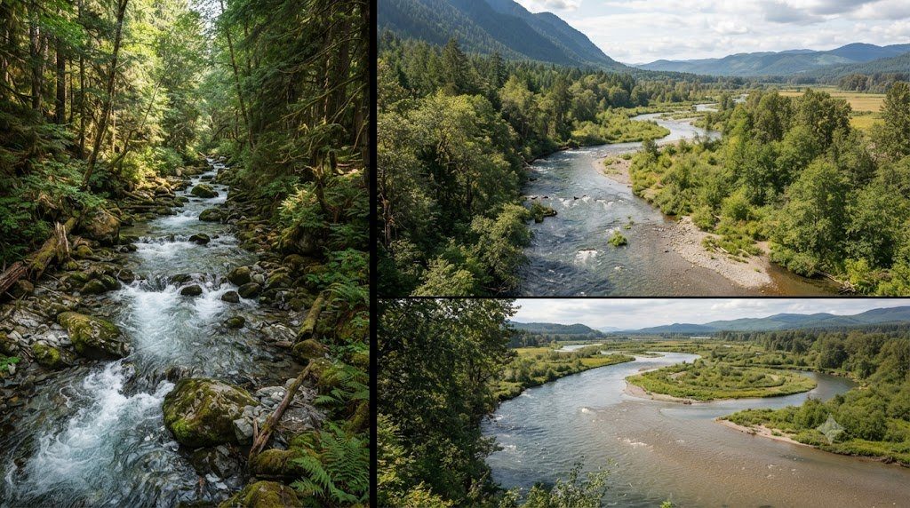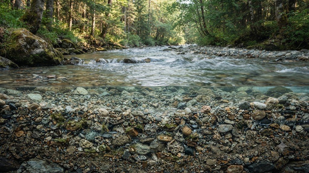
If you look at a gravel-bed river on a summer afternoon, you might assume that the entire ecosystem is contained within the surface water visible between the banks. In reality, a river is a three-dimensional entity: beneath the cobble bed and extending dozens of meters laterally beneath the riparian gravel terraces lies the Hyporheic Zone (from the Greek hypo, under, and rheos, flow). The hyporheic zone is the subterranean ecotone where surface stream water continuously infiltrates into porous alluvial sediments, mixes with regional groundwater, and upwells back into the open channel.
Often referred to as the ‘liver of the river’, the hyporheic zone performs critical ecosystem services: filtering organic particulates, driving rapid microbial nutrient transformations (such as nitrification and denitrification), buffering extreme water temperatures, and providing an underground refuge (the hyporheos) for specialized benthic organisms and developing fish embryos. In this monograph, we explore the hydrodynamic drivers of hyporheic exchange, redox biogeochemistry, and interstitial bioindicators.
Hydrodynamic Drivers of Hyporheic Exchange Flow
Why does surface river water drive downward into the porous gravel bed rather than simply flowing down the open channel? Hyporheic exchange is governed by hydraulic head gradients created by bed topography and channel curvature:
- Pool-Riffle Longitudinal Pressure Heads: As water accelerates over the crest of a gravel riffle, the water surface drops, creating high hydrostatic pressure upstream of the riffle crest. This forces surface water downward into the streambed (downwelling). As the subsurface water travels through the gravel under the riffle toward the low-pressure pool downstream, it re-emerges through the gravel bed (upwelling).
- Obstruction-Induced Pumping (Large Woody Debris & Boulders): When fast-moving lotic flow strikes an immovable boulder or submerged log jam, stagnation pressure forces water down into the permeable sediments beneath the obstruction, exiting as an upwelling jet on the leeward side.
- Meander Neck Short-Circuiting: On a sinuous river bend, the hydraulic gradient across the narrow neck of an alluvial meander is far steeper than the gradient along the winding channel loop. Surface water downwells on the upstream bank, travels straight through the subterranean gravels, and upwells on the downstream bank.
Measuring Hyporheic Flow: Piezometers and Conservative Tracers
Hydrogeologists quantify hyporheic exchange using drive-point mini-piezometers—perforated steel tubes driven 20 to 100 cm into the bed sediment. By measuring the difference between the hydraulic head inside the piezometer and the surface water level, researchers calculate the Vertical Hydraulic Gradient (VHG): a positive VHG indicates upward discharge (upwelling), while a negative VHG indicates downward recharge (downwelling). Additionally, injecting conservative chemical tracers (such as sodium bromide or rhodamine WT dye) into the surface stream allows hydrologists to model transient storage dynamics via one-dimensional advection-dispersion equations.
Biogeochemical Redox Cascades in Subsurface Sediments
As oxygenated surface water carrying dissolved organic carbon (DOC) downwells into the dark hyporheic interstitial pores, microbial biofilms coat the surface of every gravel grain. As this interstitial water moves along subterranean flow paths, microbes systematically consume electron acceptors in a predictable thermodynamic sequence:
| Interstitial Zone Depth / Flowpath | Dissolved Oxygen (DO) | Redox Potential (Eh) | Dominant Microbial Pathway | Biogeochemical Transformation |
|---|---|---|---|---|
| Upper Interstitial Boundary (0–5 cm) | High (6 to 10 mg/L) | +400 to +600 mV | Aerobic Respiration & Nitrification | Oxidizes DOC to CO2; converts NH4+ to NO3- (Nitrate) |
| Suboxic Transition Zone (5–15 cm) | Low (0.5 to 2.0 mg/L) | +200 to +400 mV | Microaerophilic Mineral Oxidation | Precipitation of Manganese and Iron Oxyhydroxides |
| Anoxic Hyporheic Core (15–50+ cm) | Anoxic (< 0.2 mg/L) | +100 to -100 mV | Denitrification (Facultative anaerobes) | Reduces NO3- to harmless atmospheric N2 gas! |
| Deep Hyporheic / Aquifer Contact | Zero DO (Strict Anoxia) | -100 to -250 mV | Iron & Sulfate Reduction | Reduces Fe(III) to soluble Fe(II); generates trace H2S |
| Methanogenic Hotspots (Pockets) | Zero DO | < -250 mV | Methanogenesis (Archaea) | Converts acetate and CO2 to methane (CH4) |
The Interstitial Biota: Hyporheos Ecology and Stygofauna
The subterranean pores between gravel grains are inhabited by a diverse, specialized ecological community known as the hyporheos:
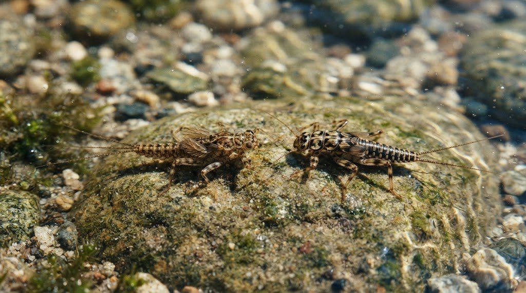
- Amphibionts (Occasional Hyporheos): Early-instar nymphs of surface stoneflies (Plecoptera, such as Leuctra) and mayflies that burrow deep into gravels to escape high-temperature summer heatwaves, anchor against scouring floods, and avoid predatory fish before returning to the open channel as mature larvae.
- Stygobites (Obligate Subterranean Fauna): Blind, unpigmented, ancient crustacean lineages—including bathynellaceans, syncarids, and blind amphipods (such as Stygobromus)—that complete their entire life cycles deep within alluvial aquifers without ever encountering sunlight.
Anthropogenic Threats: Fine Sediment Siltation and Hyporheic Clogging
The greatest threat to hyporheic ecological function is colmation (bed siltation). Agricultural runoff, clear-cut logging, and urban construction generate massive loads of fine clay and silt. When fine particles settle onto gravel beds, they infiltrate into the interstitial pores, creating an impermeable mud seal that cuts off downwelling surface water. Deprived of oxygenated flow, the gravel bed turns black, sulfurous, and anoxic—smothering developing fish eggs, killing interstitial bioindicators, and eliminating the river’s capacity to naturally denitrify agricultural runoff.
Solute Transport Modeling: Transient Storage Equations (OTIS Model)
In classical one-dimensional advection-dispersion modeling, solute transport assumes all water moves forward down the channel. However, when conservative tracers (such as bromide or rhodamine) are injected into a natural river, breakthrough curves display long, asymmetric ‘tails’—proving that a significant volume of water is temporarily delayed in stagnant zones before rejoining the main flow. This behavior is mathematically modeled using the USGS One-Dimensional Transport with Inflow and Storage (OTIS) model:
∂C / ∂t = -u * (∂C / ∂x) + DL * (∂2C / ∂x2) + α * (Cs – C)
∂Cs / ∂t = -α * (A / As) * (Cs – C)
Where $C$ is main-channel solute concentration, $C_s$ is solute concentration in the storage zone, $A$ is channel cross-sectional area, $A_s$ is the cross-sectional area of the hyporheic/transient storage zone, and $\alpha$ is the interstitial exchange coefficient ($1/s$). Sinuous gravel-bed streams with high $A_s / A$ ratios (>0.4) possess enormous subsurface retention capacity, transforming dissolved pollutants into biomass far more effectively than straightened agricultural ditches.
Hyporheic Biomonitoring: Deploying Freeze-Coring for Interstitial Integrity
To sample the delicate sediment-pore interface without collapsing interstitial gravel structures, researchers deploy liquid nitrogen or liquid carbon dioxide Freeze-Cores: a hollow copper tube is driven 60 cm into the streambed, and liquid coolant is poured down the interior. Over 15 minutes, a 20-pound frozen cylinder of gravel, pore water, organic biofilms, and interstitial organisms freezes solidly to the outside of the probe, allowing perfect laboratory vertical dissection of hyporheic siltation layers.
Salmonid Spawning Redd Micro-Hydraulics and Interstitial Gas Exchange
The survival of embryonic salmon, trout, and charr is intimately bound to the micro-hydraulics of the hyporheic zone. When an adult female salmonid excavates her spawning nest (a redd) in a clean gravel riffle, her vigorous tail flappings create a clean gravel mound flanked by an upstream depression (the pit). This engineered gravel topography generates a localized hydrostatic pressure gradient that forces oxygen-rich surface river water down through the porous gravels directly across the buried fertilized eggs.
For embryos to survive the 60-to-120-day incubation period inside the dark gravel bed, the interstitial apparent velocity ($v_a$) of hyporheic pore water must exceed at least 0.5 to 1.0 millimeters per second, delivering fresh dissolved oxygen ($> 8.0 \text{ mg/L}$) while flushing away toxic metabolic wastes (ammonia and carbon dioxide). If fine agricultural siltation clogs the gravel interstitial pore spaces by even 15% to 20%, hyporheic flow stalls, dissolved oxygen collapses, and 90% to 100% of the developing embryos suffocate before hatching—demonstrating why protecting the hyporheic zone is critical for continental fisheries.
Pharmaceutical and Pesticide Attenuation in Interstitial Biofilms
Emerging scientific research reveals that the hyporheic zone acts as a formidable biogeochemical barrier against synthetic micropollutants. When municipal wastewater effluent carrying human pharmaceuticals (such as ibuprofen, diclofenac, carbamazepine, and antibiotics) and agricultural neonicotinoid pesticides travels down a river, hyporheic exchange circulates these compounds through dense microbial biofilms coating gravel grains. Through prolonged contact time with diverse extracellular enzymes (such as laccases and peroxidases) in alternating aerobic and anoxic micro-niches, up to 70% of dissolved pharmaceutical residues are biodegraded or co-metabolically transformed, purifying river water naturally.
Field Hydrometry Protocols and Annual Catchment Survey Schedule
Field implementation of The Hyporheic Zone in a working river basin requires disciplined adherence to standardized hydrometry protocols. Stream channels exhibit profound temporal variability: baseflow conditions in late summer expose low-flow hydraulic geometries, while spring snowmelt and autumn convective storms mobilize bedload sediment and reshape gravel bars.
A professional lotic monitoring program coordinates cross-sectional surveying, velocity gauging, bed material pebble counts, and continuous water quality logging across four distinct hydrological stages. Use the operational field matrix below to align river surveys with annual hydrograph dynamics.
| Hydrological Stage | Flow Regime & Stage Height | Channel Energy & Hydraulic Focus | Mandatory Field Survey Protocol | Critical Safety & QA/QC Precautions |
|---|---|---|---|---|
| Early Spring Freshet | High Stage / Snowmelt Peak | Near Bankfull (High bed shear tau_0) | Deploy bridge-mounted ADCP or cableway winch for peak discharge Q | Never wade swift water; tether boat rigs; verify velocity sensor calibration |
| Post-Flood Late Spring | Receding Bankfull to Med Flow | Sediment sorting & bar deposition | Survey cross-sectional geometry at monumented pins; assess bank erosion BEHI | Inspect benchmark datum elevations; check monument stability against scour |
| Summer Baseflow (Dry Period) | Low Stage / Groundwater Fed | Subcritical tranquil flow (Fr < 0.3) | Perform 100-particle Wolman pebble counts; sample benthic macroinvertebrates | Wade along riffle transects; inspect periphyton cover; calibrate optical DO |
| Autumn Storm Pulses | Flash Stage Rises (Rain events) | Transient storage & organic drift | Measure suspended sediment concentration (SSC) & turbidity sonde spikes | Clean optical wiper blades on multi-parameter sondes; check solar battery voltage |
Wolman Pebble Count Standardization for Streambed Particle Sizing
Bed material size distribution ($D_{50}$, $D_{84}$) governs roughness, sediment mobility, and spawning gravel quality. To execute an unbiased Wolman Pebble Count (Wolman, 1954) across a representative riffle reach:
- Blind Sampling Geometry: Step along a zig-zag transect across the active bankfull channel. At each step, avert your eyes, reach down with your index finger at the tip of your boot, and retrieve the first particle your finger touches.
- Measuring the Intermediate Axis (b-axis): Measure the particle’s intermediate dimension ($b$-axis—neither the longest length nor the thinnest thickness) using a gravelometer template or precision caliper to the nearest millimeter.
- Cumulative Frequency Distribution (100 Particles Minimum): Tally particles into standard Wentworth size classes (<2mm silt/sand, 2–4mm, 4–8mm, up to >256mm boulders). Plot grain size on a log scale against cumulative percent finer to extract $D_{16}$, $D_{50}$ (median diameter), and $D_{84}$ for shear stress modeling.
Frequently Asked Questions Concerning Fluvial Dynamics & River Science
Why is bankfull discharge considered the most effective geomorphic flow?
While rare 100-year catastrophic floods move enormous boulders, they occur so infrequently that their cumulative geological work is limited. Conversely, everyday baseflows occur constantly but lack the shear stress required to move gravel. Bankfull discharge (occurring roughly every 1.5 years) balances moderate frequency with high sediment-transport capacity, performing the highest percentage of total annual bedload movement and sculpting permanent channel dimensions.
How does large woody debris (LWD) benefit stream hydraulics?
Large fallen trees and root wads increase channel boundary roughness, dissipating excess flood energy and preventing downstream bed incision. Furthermore, water flowing around log jams scours out deep, cold plunge pools that provide critical summer thermal refugia for trout and salmon while creating stable depositional gravel beds for spawning.
What is the difference between suspended load and bedload?
Suspended load consists of fine clays and silts held aloft in the water column by turbulent fluid eddies, traveling at nearly the same velocity as the flowing water. Bedload consists of coarse sands, gravels, and cobbles that roll, slide, and bounce (saltate) along the streambed, moving intermittently only when critical bed shear stress exceeds the Shields threshold.