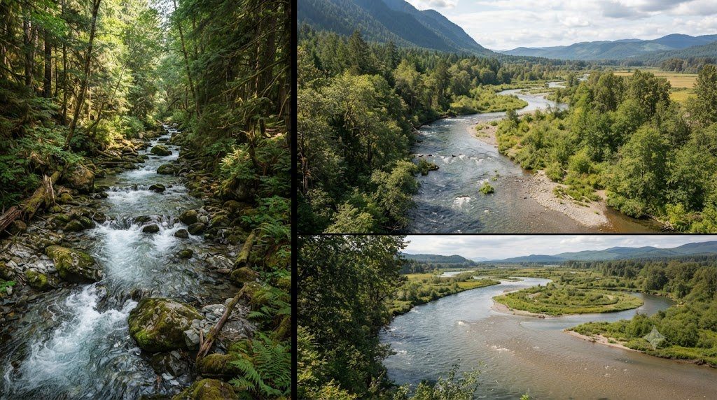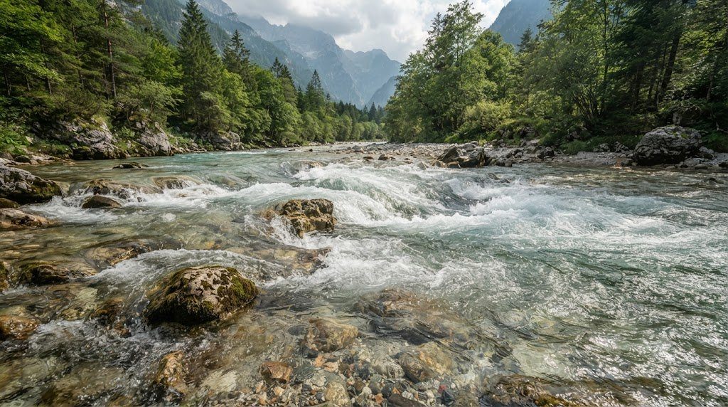
Every physical feature of a natural river—from the deep, languid pools where trout seek thermal refuge to the turbulent, oxygenating white-water riffles where caddisflies anchor their nets—is an equilibrium expression of open-channel hydraulics. Unlike closed conduits where liquid moves under pressurized mechanical boundaries, open-channel flow occurs with a free liquid surface exposed directly to atmospheric pressure, driven entirely by the downslope component of gravitational acceleration.
Understanding how water navigates natural channel geometries requires mastering the physical laws that govern boundary layer friction, bed shear stress, turbulent boundary velocity profiles, and sediment transport mechanics. In this advanced hydrological treatise, we analyze Manning’s roughness equation, the Froude number, Shields’ threshold parameter for bedload entrainment, and the dynamics of channel-forming bankfull discharge.
Manning’s Empirical Formula and Channel Flow Resistance
Formulated by Irish engineer Robert Manning in 1889, Manning’s Equation remains the standard mathematical workhorse for calculating cross-sectional average velocity and volumetric discharge in uniform, steady open channels:
V = (1.0 / n) * R^(2/3) * S^(1/2) [SI Metric Units]
Where:
- V: Cross-sectional mean flow velocity (meters per second, m/s).
- n: Manning’s roughness coefficient (dimensionless empirical parameter reflecting boundary frictional resistance).
- R: Hydraulic radius (meters, m), defined as cross-sectional flow area ($A$) divided by the wetted perimeter ($P$): $R = A / P$.
- S: Energy slope or longitudinal channel bed gradient (dimensionless, meters drop per meter length, m/m).
Volumetric discharge ($Q$, in cubic meters per second, $m^3/s$ or cusecs) is directly calculated via the continuity equation: $Q = V \cdot A$.
Quantifying Manning’s Roughness Coefficient (n) in Natural Channels
In smooth, concrete-lined stormwater canals, Manning’s $n$ is very low (~0.012 to 0.015). In natural streams, however, boundary roughness is vastly higher due to bed sediment grain sizes, banks irregular geometry, large woody debris (LWD), and seasonal aquatic vegetation. Stream hydrologists estimate natural roughness using Cowan’s additive method ($n = (n_0 + n_1 + n_2 + n_3 + n_4) \cdot m_5$), which accounts for bed material, surface irregularities, channel shape variations, obstructions, and meander tortuosity.
Boundary Shear Stress and Shields’ Critical Mobility Parameter
Water flowing across an alluvial riverbed exerts a tangential dragging force known as Bed Shear Stress ($\tau_0$). In steady, uniform open-channel flow, average boundary shear stress is mathematically derived from the depth-slope product:
τ0 = ρ * g * R * S
Where $\rho$ is water density ($1000 \text{ kg/m}^3$), $g$ is gravitational acceleration ($9.81 \text{ m/s}^2$), $R$ is hydraulic radius (or mean depth $D$ in wide channels), and $S$ is energy slope. Shear stress is measured in Pascals ($N/m^2$).
| Channel Bed Sediment Class | Median Grain Size (D50) | Manning’s Roughness (n) | Critical Shear Stress (τc) | Sediment Transport Mechanism |
|---|---|---|---|---|
| Silt and Fine Clay | < 0.062 mm | 0.020 – 0.030 | 0.1 to 0.5 Pa | Permanent Suspended Load / Wash Load |
| Medium to Coarse Sand | 0.25 to 2.0 mm | 0.025 – 0.035 | 0.2 to 1.8 Pa | Intermittent Suspension & Saltation |
| Fine to Coarse Gravel | 4.0 to 32 mm | 0.030 – 0.045 | 3.0 to 25.0 Pa | Bedload Rolling, Sliding, and Saltation |
| Cobbles (Stream Riffles) | 64 to 256 mm | 0.045 – 0.070 | 50.0 to 200.0 Pa | Bedload Mobilization at Bankfull Discharge |
| Boulders (High-Gradient Mountain) | > 256 mm | 0.070 – 0.150+ | > 220.0 Pa | Extreme Flood Immobility / Structural Steps |
Shields’ Diagram and the Incipient Motion of Gravel
When does an individual grain of gravel on a stream bed begin to roll? In 1936, Albert F. Shields established the dimensionless parameter governing incipient sediment motion:
τ* = τ0 / [(ρs – ρ) * g * D]
Where $\rho_s$ is sediment density (typically $2650 \text{ kg/m}^3$ for quartz), and $D$ is the sediment grain diameter. When the dimensionless shear stress $\tau^*$ exceeds the critical threshold (typically $\tau_c^* \approx 0.045$ to $0.060$ for turbulent gravel beds), the hydrodynamic drag and lift forces exceed the submerged gravitational friction of the stone, initiating bedload transport.
The Froude Number: Subcritical vs. Supercritical Open-Channel Flow
The hydrodynamic state of open-channel flow is governed by the Froude Number ($Fr$), a dimensionless ratio comparing inertial kinetic forces to gravitational wave propagation forces:
Fr = V / √(g * D)
Where $V$ is mean velocity and $D$ is hydraulic depth:
- Subcritical Flow ($Fr < 1.0$): Known as ‘tranquil’ or ‘streaming’ flow. Gravitational wave speed exceeds flow velocity, meaning surface disturbance ripples can propagate upstream. Most lowland rivers and deep stream pools operate in subcritical flow.
- Critical Flow ($Fr = 1.0$): Flow energy is at its absolute thermodynamic minimum for a given discharge. Surface waves are held stationary.
- Supercritical Flow ($Fr > 1.0$): Known as ‘rapid’ or ‘shooting’ flow. Flow velocity exceeds gravity wave propagation velocity, meaning surface waves cannot travel upstream. Supercritical flow occurs over steep spillways, mountain torrent chutes, and dam overflow crests. When supercritical flow abruptly transitions back into subcritical flow, it creates a turbulent Hydraulic Jump that dissipates enormous kinetic energy.
Bankfull Discharge: The Channel-Forming Effective Flow
A common misconception is that the catastrophic 100-year flood shapes the geometry of river channels. In reality, quantitative sediment budgets reveal that the Bankfull Discharge ($Q_{bkf}$)—the flow that completely fills the active channel to the brink of overflowing onto its active floodplain, typically recurring every 1.2 to 1.8 years (recurrence interval $RI \approx 1.5$ years)—performs the vast majority of cumulative geomorphic work. Because bankfull flows occur with moderate frequency and exert sufficient shear stress to mobilize the bedload, natural channel design engineers calibrate all stream restoration dimensions to the bankfull stage.
Turbulent Boundary Layer Kinematics and the Law of the Wall
Within the open channel cross-section, velocity is never uniformly distributed. Due to molecular viscosity and turbulent momentum exchange against the stationary bed and banks, a distinct turbulent boundary layer develops. In fully turbulent open-channel flow over rough gravel beds ($Re_* > 70$), the vertical velocity profile follows the universal Prandtl-von Kármán Law of the Wall (the logarithmic velocity profile):
u(z) = (u* / κ) * ln(z / z0)
Where $u(z)$ is the local flow velocity at height $z$ above the streambed, $\kappa$ is the universal von Kármán constant (approximately 0.40 for clear water), $z_0$ is the hydrodynamic roughness height ($z_0 \approx D_{84} / 30$ in gravel beds), and $u^*$ is the shear velocity (friction velocity), defined as:
u* = √(τ0 / ρ) = √(g * R * S)
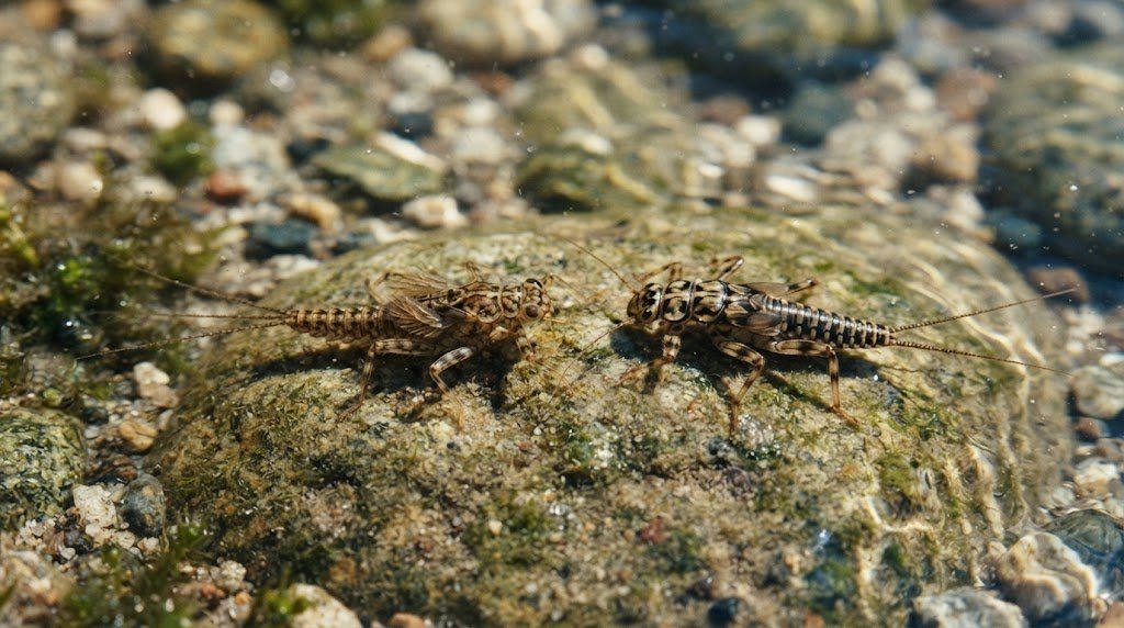
This logarithmic relationship explains why benthic organisms living in the lowest few millimeters of the bed experience dramatically reduced flow velocities compared to the surging torrent overhead, allowing flatheaded mayflies and water pennies to anchor safely inside the viscous sublayer.
Acoustic Doppler Current Profiler (ADCP) Field Discharge Transects
Modern USGS hydrological gauging stations and river researchers have largely transitioned from manual mechanical Price AA cup meters to Acoustic Doppler Current Profilers (ADCP). Mounted on a trimaran tethered to a bridge or remote-controlled boat, an ADCP transmits ultrasonic acoustic pulses (typically 600 kHz to 3.0 MHz) down into the water column. By measuring the Doppler frequency shift reflected off microscopic suspended particles, the instrument maps thousands of discrete velocity vectors across hundreds of depth cells (‘bins’) simultaneously, integrating three-dimensional channel discharge ($Q$) to an accuracy of $\pm 1.5\%$ in minutes.
Sediment Rating Curves and Bedload Hysteresis Loops
During a major storm hydrograph, sediment transport is rarely symmetrical between the rising and falling limbs of the flood wave. Hydrogeologists quantify this phenomenon through Sediment Rating Curves ($Q_s = a \cdot Q^b$) and Sediment Hysteresis Loops. When storm runoff accelerates down an urbanized or agricultural watershed, loose surface soil particles and easily erodible bank fines are mobilized immediately on the rising limb of the hydrograph, causing Suspended Sediment Concentrations (SSC) to peak several hours before peak water discharge—generating a characteristic Clockwise Hysteresis Loop.
Conversely, in well-vegetated montane catchments where sediment supply is limited to slow headwater mass-wasting or channel bank slumping, peak sediment concentration often lags behind peak discharge, producing a Counter-Clockwise Hysteresis Loop. Accurately modeling these dynamic hysteretic loops is vital for reservoir silting calculations, dredging schedules, and predicting the suffocation of salmonid gravel spawning redds beneath fine silt plumes.
HEC-RAS Hydraulic Modeling: 1D Steady vs. 2D Unsteady Flood Inundation
Modern river engineering relies on numerical hydrodynamic modeling packages developed by the US Army Corps of Engineers (USACE), specifically HEC-RAS (Hydrologic Engineering Center’s River Analysis System). While traditional 1D steady-state step-backwater models solve the standard energy equation ($z_1 + y_1 + \alpha_1 V_1^2 / 2g = z_2 + y_2 + \alpha_2 V_2^2 / 2g + h_e$) between surveyed cross-sections, complex natural floodplains demand 2D unsteady shallow water equations (Saint-Venant equations). Two-dimensional models compute diffusion-wave and full-momentum velocity vectors across irregular digital elevation terrain grids, revealing localized eddy recirculation zones, cutbank shear stress hotspots, and bridge abutment scour hazards that 1D models completely miss.
Field Hydrometry Protocols and Annual Catchment Survey Schedule
Field implementation of Open-Channel Fluvial Hydraulics in a working river basin requires disciplined adherence to standardized hydrometry protocols. Stream channels exhibit profound temporal variability: baseflow conditions in late summer expose low-flow hydraulic geometries, while spring snowmelt and autumn convective storms mobilize bedload sediment and reshape gravel bars.
A professional lotic monitoring program coordinates cross-sectional surveying, velocity gauging, bed material pebble counts, and continuous water quality logging across four distinct hydrological stages. Use the operational field matrix below to align river surveys with annual hydrograph dynamics.
| Hydrological Stage | Flow Regime & Stage Height | Channel Energy & Hydraulic Focus | Mandatory Field Survey Protocol | Critical Safety & QA/QC Precautions |
|---|---|---|---|---|
| Early Spring Freshet | High Stage / Snowmelt Peak | Near Bankfull (High bed shear tau_0) | Deploy bridge-mounted ADCP or cableway winch for peak discharge Q | Never wade swift water; tether boat rigs; verify velocity sensor calibration |
| Post-Flood Late Spring | Receding Bankfull to Med Flow | Sediment sorting & bar deposition | Survey cross-sectional geometry at monumented pins; assess bank erosion BEHI | Inspect benchmark datum elevations; check monument stability against scour |
| Summer Baseflow (Dry Period) | Low Stage / Groundwater Fed | Subcritical tranquil flow (Fr < 0.3) | Perform 100-particle Wolman pebble counts; sample benthic macroinvertebrates | Wade along riffle transects; inspect periphyton cover; calibrate optical DO |
| Autumn Storm Pulses | Flash Stage Rises (Rain events) | Transient storage & organic drift | Measure suspended sediment concentration (SSC) & turbidity sonde spikes | Clean optical wiper blades on multi-parameter sondes; check solar battery voltage |
Wolman Pebble Count Standardization for Streambed Particle Sizing
Bed material size distribution ($D_{50}$, $D_{84}$) governs roughness, sediment mobility, and spawning gravel quality. To execute an unbiased Wolman Pebble Count (Wolman, 1954) across a representative riffle reach:
- Blind Sampling Geometry: Step along a zig-zag transect across the active bankfull channel. At each step, avert your eyes, reach down with your index finger at the tip of your boot, and retrieve the first particle your finger touches.
- Measuring the Intermediate Axis (b-axis): Measure the particle’s intermediate dimension ($b$-axis—neither the longest length nor the thinnest thickness) using a gravelometer template or precision caliper to the nearest millimeter.
- Cumulative Frequency Distribution (100 Particles Minimum): Tally particles into standard Wentworth size classes (<2mm silt/sand, 2–4mm, 4–8mm, up to >256mm boulders). Plot grain size on a log scale against cumulative percent finer to extract $D_{16}$, $D_{50}$ (median diameter), and $D_{84}$ for shear stress modeling.
Frequently Asked Questions Concerning Fluvial Dynamics & River Science
Why is bankfull discharge considered the most effective geomorphic flow?
While rare 100-year catastrophic floods move enormous boulders, they occur so infrequently that their cumulative geological work is limited. Conversely, everyday baseflows occur constantly but lack the shear stress required to move gravel. Bankfull discharge (occurring roughly every 1.5 years) balances moderate frequency with high sediment-transport capacity, performing the highest percentage of total annual bedload movement and sculpting permanent channel dimensions.
How does large woody debris (LWD) benefit stream hydraulics?
Large fallen trees and root wads increase channel boundary roughness, dissipating excess flood energy and preventing downstream bed incision. Furthermore, water flowing around log jams scours out deep, cold plunge pools that provide critical summer thermal refugia for trout and salmon while creating stable depositional gravel beds for spawning.
What is the difference between suspended load and bedload?
Suspended load consists of fine clays and silts held aloft in the water column by turbulent fluid eddies, traveling at nearly the same velocity as the flowing water. Bedload consists of coarse sands, gravels, and cobbles that roll, slide, and bounce (saltate) along the streambed, moving intermittently only when critical bed shear stress exceeds the Shields threshold.