Beneath the surface topography of continents lies Earth’s vastest accessible freshwater reservoir: groundwater. Containing over 98% of the liquid freshwater on our planet, groundwater sustains global agricultural irrigation, provides drinking water for billions of people, and maintains baseflow in rivers during prolonged droughts. Yet groundwater does not flow in wide, open subterranean caverns (except in rare karst formations); it moves slowly through microscopic pore channels between sand grains, gravel deposits, and micro-fractures in crystalline bedrock.
The foundational physics governing subsurface fluid flow was formulated in 1856 by French civil engineer Henry Darcy while designing municipal sand filtration basins for the city of Dijon: Darcy’s Law. Darcy’s empirical relationship transformed hydrogeology from guesswork into an exact mathematical science. In this technical monograph, we deconstruct Darcy’s flux equation, the physics of hydraulic conductivity ($K$), transmissivity ($T$), and the analytical solutions of Theis and Cooper-Jacob aquifer pumping tests.
Mathematical Formulation of Darcy’s Law and Seepage Velocity
Darcy demonstrated that volumetric flow rate through a porous medium is directly proportional to cross-sectional area and hydraulic head loss, and inversely proportional to the flow path length:
Q = -K * A * (dh / dl) = -K * A * i
Where:
- Q: Volumetric discharge ($m^3/s$ or $m^3/day$).
- K: Hydraulic conductivity ($m/s$ or $m/day$), representing the ease with which fluid moves through the pore matrix.
- A: Total cross-sectional area perpendicular to flow ($m^2$).
- i = dh / dl: Hydraulic gradient (dimensionless, meters head loss per meter of distance, $m/m$). The negative sign indicates flow occurs in the direction of decreasing hydraulic head.
Darcy Flux (q) vs. True Linear Seepage Velocity (vs)
A critical point of confusion in groundwater engineering is the difference between specific discharge (Darcy Flux, $q$) and true groundwater seepage velocity ($v_s$). The Darcy flux ($q = Q / A = K \cdot i$) assumes water moves through 100% of the cross-sectional area. In reality, solid mineral grains occupy most of the space! Water can only flow through the interconnected pore voids. Therefore, true linear pore velocity is calculated by dividing Darcy flux by the effective porosity ($n_e$) of the medium:
vs = q / ne = (K * i) / ne
Because effective porosity in sands is typically 0.20 to 0.30, actual contaminant plumes and water molecules travel 3 to 5 times faster than the simple Darcy velocity!
Hydraulic Conductivity (K) Across Geological Formations
Hydraulic conductivity spans an astonishing twelve orders of magnitude across Earth’s geologic strata, reflecting the extreme heterogeneity of subterranean matrices:
| Geological Material / Matrix | Hydraulic Conductivity K (m/s) | Hydraulic Conductivity K (m/day) | Effective Porosity (ne) | Hydrogeological Function |
|---|---|---|---|---|
| Clean Coarse Gravel | 10^(-2) to 10^(-1) | 800 to 8,000+ | 0.25 to 0.35 | Prolific Aquifer (Extremely high yield) |
| Coarse to Medium Sand | 10^(-4) to 10^(-2) | 8 to 800 | 0.20 to 0.30 | Major Commercial / Municipal Aquifer |
| Fine Sand and Loess | 10^(-5) to 10^(-4) | 0.8 to 8 | 0.15 to 0.25 | Moderate Aquifer / Domestic Wells |
| Silt and Silty Sand | 10^(-7) to 10^(-5) | 0.008 to 0.8 | 0.05 to 0.15 | Aquitard (Semi-confining leaky layer) |
| Dense Clay / Glacial Till | 10^(-11) to 10^(-8) | 10^(-6) to 0.0008 | 0.01 to 0.05 | Aquiclude (Virtually impermeable seal) |
| Unfractured Crystalline Bedrock | < 10^(-12) | < 10^(-7) | < 0.01 | Impermeable Basal Aquifuge |
| Karst Limestone Conduits | 10^(-2) to > 1.0 | > 800 to 80,000+ | Secondary porosity | Super-Conduit Flow (Turbulent subterranean rivers) |
Aquifer Parameters: Transmissivity (T) and Storativity (S)
When modeling real-world confined and unconfined aquifers, hydrogeologists upscale hydraulic conductivity to two fundamental macroscopic parameters:
- Transmissivity ($T$): The rate at which water is transmitted through a unit width of the entire saturated thickness ($b$) of an aquifer under a unit hydraulic gradient: $T = K \cdot b$ ($m^2/s$ or $m^2/day$). High transmissivity (>500 $m^2/day$) indicates a world-class municipal water source.
- Storativity (Storage Coefficient, $S$): The volume of water an aquifer releases from storage per unit surface area per unit decline in hydraulic head. In confined aquifers, water is released purely via mineral matrix decompression and water expansion, resulting in very low storativity ($S = 10^{-5}$ to $10^{-3}$). In unconfined aquifers, water is released by physical gravity drainage of pore voids, represented by the Specific Yield ($S_y = 0.10$ to $0.30$).
Aquifer Pumping Tests: The Theis Non-Equilibrium Equation
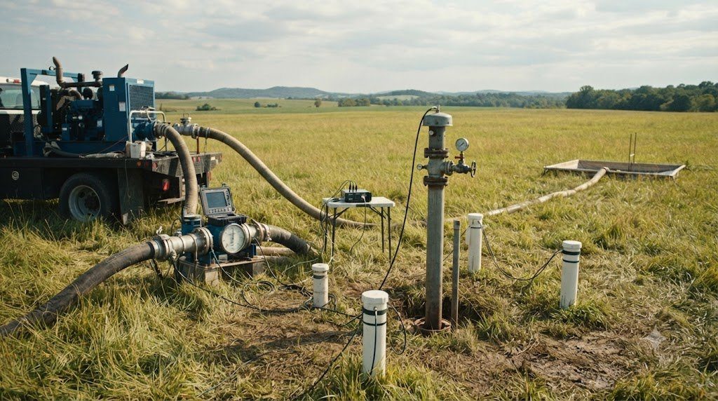
To determine $T$ and $S$ in the field, hydrogeologists conduct a controlled Aquifer Pumping Test. A central extraction well is pumped at a constant discharge rate ($Q$), while water level drawdowns ($s$) are monitored continuously in surrounding observation wells at radius $r$. In 1935, Charles V. Theis solved the transient radial flow equation by analogy to heat conduction:
s = [Q / (4 * π * T)] * W(u)
Where $W(u)$ is the Theis Well Function evaluated at $u = (r^2 \cdot S) / (4 \cdot T \cdot t)$. By plotting field drawdown versus time on log-log graph paper and curve-matching against the theoretical Theis type curve (or using Cooper-Jacob semi-log straight-line approximations for small $u < 0.05$), engineers calculate exact transmissivity and storativity values, predicting decades of sustainable well-field pumping capacity.
Laboratory Permeameter Testing: Constant-Head vs. Falling-Head Protocols
Before drilling multi-million-dollar well fields, geotechnical hydrogeologists measure the hydraulic conductivity ($K$) of geological core samples in the laboratory using standardized permeameter cells:
- Constant-Head Permeameter (For High-K Coarse Sands and Gravels): Water is passed through a cylindrical soil sample of length $L$ and area $A$ under a constant hydraulic head difference ($\Delta h$). By measuring the outflow volume ($V$) over time ($t$), hydraulic conductivity is calculated directly: $K = (V \cdot L) / (A \cdot t \cdot \Delta h)$.
- Falling-Head Permeameter (For Low-K Silts and Clays): Connected to a narrow vertical standpipe tube of area $a$. Water level in the standpipe drops from $h_0$ to $h_1$ over time $t$ as water seeps through the tight soil core: $K = [a \cdot L / (A \cdot t)] \cdot \ln(h_0 / h_1)$.
The Cooper-Jacob Semi-Log Approximation for Pumping Tests
For pumping tests where the dimensionless parameter $u = (r^2 \cdot S) / (4 \cdot T \cdot t)$ is small ($u < 0.05$, representing long pumping times or small distances from the well), H.H. Cooper and C.E. Jacob simplified the complex Theis exponential integral into a straight-line semi-log relationship:
s = [2.303 * Q / (4 * π * T)] * log10(2.25 * T * t / [r2 * S])
By plotting drawdown ($s$) on an arithmetic y-axis against time ($t$) on a logarithmic x-axis, the slope of the line across one full log cycle of time ($\Delta s$) yields transmissivity directly: $T = (2.303 \cdot Q) / (4 \cdot \pi \cdot \Delta s)$!
Slug Testing: Hvorslev and Bouwer-Rice Analytical Solutions
When conducting site contamination investigations, operating an 8-hour high-yield pumping test is often prohibitively expensive or illegal due to hazardous disposal regulations for pumped contaminated water. Instead, hydrogeologists measure localized hydraulic conductivity ($K$) using rapid Slug Tests (Single-Well Response Tests):
A solid, sealed mechanical cylinder (‘slug’) of known volume is instantly submerged into the monitoring well (or removed), causing an instantaneous rise (falling-head slug test) or drop (rising-head slug test) in water level. As water levels recover toward static equilibrium, a high-frequency pressure transducer records recovery head ($h$) every 0.25 seconds. Hydrogeologists analyze the data using:
- The Hvorslev Method (1951): Applied to confined piezometers: $K = [r^2 \cdot \ln(L / R)] / [2 \cdot L \cdot T_0]$, where $r$ is well casing radius, $R$ is borehole screen radius, $L$ is screen intake length, and $T_0$ is the basic time lag extracted from semi-log recovery plots.
- The Bouwer and Rice Method (1976): Designed specifically for unconfined water-table wells, accounting for the free surface boundary and non-linear flow geometry surrounding the partially submerged screen.
Scale Dependency of Hydraulic Conductivity
Hydrogeologists must always recognize the Scale Effect of Hydraulic Conductivity. Laboratory permeameter tests on small 5-centimeter core samples measure small-scale matrix pores, typically yielding low $K$ values. Field slug tests (interrogating 1 to 2 meters around a well) yield moderate $K$ values. Full-scale multi-day pumping tests (interrogating thousands of square meters) yield significantly higher $K$ values because large-scale pumping intercepts interconnected high-permeability sand lenses, macropores, and fractures that small core samples inevitably miss.
Monitoring Well Drilling, Development, and Hydrogeological Sampling
Validating the hydrogeological principles of Darcy’s Law and Hydraulic Conductivity requires installing, developing, and sampling certified groundwater monitoring wells. If a monitoring well is drilled with inappropriate muds or sampled using high-flow pumps that aerate the water, dissolved volatile organic compounds (VOCs) strip out and dissolved metals precipitate onto casing walls, generating invalid laboratory data.
A professional hydrogeological investigation follows strict EPA and USGS low-flow purge protocols to ensure that water extracted from the borehole represents true, undisturbed aquifer conditions. Use the well development and sampling matrix below.
| Hydrogeological Stage | Drilling Rig / Sampling Hardware | Operational Objective | Standard Field Procedure | Critical Contamination Safeguard |
|---|---|---|---|---|
| Borehole Drilling | Hollow-Stem Auger or Sonic Rig | Penetrate target saturated aquifer zone | Log lithological soil cores every 5 feet; record depth to water table | Never use bentonite drilling muds in screen zone; use clean water only |
| Well Installation | 2-inch Schedule 40 PVC; 0.010″ slotted screen | Establish permanent intake zone | Pack screen with graded 20/40 silica sand; seal above with 2ft bentonite pellet plug | Cap wellhead with locking steel protective casing bolted into concrete pad |
| Well Development | Surge block & high-capacity submersible pump | Remove drill fines & develop gravel pack | Surge and pump until turbidity drops below 10 NTU; flush at least 5 casing volumes | Prevents silting of pump impellers and ensures natural hydraulic conductivity |
| Low-Flow Purging (Low-Flow Micro-Purge) | Adjustable-rate bladder pump or peristaltic pump | Extract formation water with minimal drawdown | Pump at 100 to 500 mL/min; log pH, DO, ORP, Temp, Specific Conductance in flow cell | Purge until 3 consecutive readings over 5-minute intervals stabilize within 10% |
| Sample Collection | Direct filling of laboratory certified glass VOA vials | Capture VOCs, heavy metals, and nutrients | Fill 40 mL VOA vials to positive meniscus without headspace/bubbles; preserve with HCl | Zero air bubbles in vials; keep samples chilled at 4°C in dark cooler |
Flow-Through Cell Parameter Stabilization Criteria
During low-flow micro-purging, groundwater is pumped through an enclosed, sealed multichannel flow-through cell containing calibrated probes. Pumping continues until parameters achieve strict stabilization over three consecutive readings spaced 3 to 5 minutes apart:
- pH: Stable within $\pm 0.1 \text{ pH units}$.
- Specific Electrical Conductance: Stable within $\pm 3\%$ of reading.
- Dissolved Oxygen (DO): Stable within $\pm 10\%$ (or $\pm 0.2 \text{ mg/L}$ when $< 2.0 \text{ mg/L}$).
- Oxidation-Reduction Potential (ORP): Stable within $\pm 10 \text{ millivolts}$.
- Turbidity: Stable within $\pm 10\%$ (and ideally $< 10 \text{ NTU}$).
Frequently Asked Questions Concerning Hydrogeology & Aquifers
What is the difference between porosity and permeability?
Porosity ($\eta$) is the percentage of total rock or sediment volume occupied by open void spaces, representing how much water an earth material can hold. Permeability ($k$) is the measure of how easily fluids can flow through those voids, depending on pore size and interconnectivity. A dense clay can have high porosity (45% voids) but near-zero permeability because its microscopic pore throats are too narrow for water to move freely.
How does a cone of depression cause land subsidence?
When an extraction well pumps groundwater faster than the aquifer recharges, hydraulic head drops in a conical depression around the well. Relieved of pore water pressure ($u$), the overburden weight of overlying rock and buildings transfers directly onto the mineral skeleton, compressing compressible clay layers and causing irreversible ground collapse and surface subsidence.
Why are karst aquifers particularly vulnerable to pollution?
Standard sand aquifers filter water through microscopic pores, removing bacteria and suspended particles via physical filtration and slow biological breakdown over years. In karst limestone aquifers, water rushes through open dissolved caves and conduits at kilometers per day with zero filtration. A chemical or septic spill at a surface sinkhole travels unfiltered straight to municipal drinking water taps within hours.